The ice sheets are unraveling. At the edges of Antarctica and Greenland and across the arctic, great swaths are breaking into icebergs and miles-wide floes.
The Larsen B Antarctic ice shelf, which covered more than 1,200 square miles and was 650 feet thick, disintegrated in 2002. Six years later the nearby Wilkins ice shelf, more than 5,000 square miles, partially collapsed. They were only the latest of ice shelves to retreat or give way over the past few decades. After taking thousands of years to form, some ice shelves are falling apart in weeks.
In each case, fractures preceded failure, says Haim Waisman, a Columbia University assistant professor of Civil Engineering and Engineering Mechanics. Waisman heads a Department of Energy-supported project to improve computer simulation of land ice cracking and how global warming accelerates it. “If we can model and understand some of these fractures, maybe this can be coupled with ice sheet simulations and give a better understanding of what’s happening.”
Waisman’s project is part of ISICLES, the Ice Sheet Initiative for CLimate ExtremeS, supported by DOE’s Office of Advanced Scientific Computing Research (ASCR).
Ice sheet models have not explicitly considered ice fracture, a complex phenomenon that demands large computer resources. Yet fractures play a pivotal role in regional behavior and influence ice dynamics over larger areas in ways scientists don’t understand.
There are ice fracture models available, Waisman says, but none are definitive, failing to capture the real scenario of the ice shelf.
That’s understandable. Ice is nearly as common in the world as liquid water, yet “it has its own challenges which are different from the usual material,” Waisman says. Ice is heterogeneous, with widely varying qualities; it can be viscous, with characteristics lurking between liquid and solid; and it compresses under its own weight, so its density can vary.
The Intergovernmental Panel on Climate Change, a group of scientists from around the world charged with assessing global climate science, defines an ice sheet as land ice thick enough to hide the underlying topography. There are only three large ice sheets today: one on Greenland and the other two on Antarctica. Ice sheets can flow into ice shelves – thick slabs of floating ice extending from coastlines and often filling inlets or bays. Nearly all ice shelves are in Antarctica.
The scale of ice sheets also poses a challenge. They cover an area the size of “the entire United States and even more, and the largest ice shelf is bigger than California,” Waisman says. And modelers want the shape of their simulated ice sheets to mimic reality. “We want to do something that’s as close as possible. So we need to somehow obtain data from experimentalists on what is the real ice out there – which is a challenge by itself.”
Once researchers get an ice shelf’s material properties down, they must calculate the effects of a daunting list of environmental factors:
- Increasing temperature, including the effects of climate change, can soften ice until it fails under its own weight.
- Relatively warm seawater circulating under a floating ice shelf can thin and weaken it.
- Ocean movement subjects the ice sheet to load fatigue, similar to how repeatedly flexing a metal sheet can make it fail.
“It adds a lot of complications,” Waisman says.
Besides fractures, the researchers will model ice calving – the spectacular birth of icebergs as they break free – and the drainage of supraglacial lakes, bodies of water that form atop glaciers.
“The lakes can disappear in a matter of minutes,” Waisman says. “Essentially there’s a network of cracks that enable the water to drain,” sending millions or billions of gallons thousands of feet below the glacier’s surface. Once there, the water is believed to lubricate the interface between ice and land, accelerating the ice sheet’s slide.
Divide and conquer
The researchers will deploy some “fancy methods” to simulate fractures, Waisman says. The foundation is the finite element method (FEM), which deploys a mesh of data points to break the domain being modeled into small pieces – millions or even billions of them, depending on the level of detail and the size of the area modeled. Computers apply the laws of physics to calculate what’s happening at each point, then assemble the points together into a full picture.
Splitting the domain into small pieces makes modeling manageable, even for complex shapes. But try adding something to the picture – a crack, say.
“You need your mesh generation or those elements that you built to conform with the crack boundaries, which by itself is a task,” Waisman says. “Now imagine that these cracks keep growing and propagating. Your geometry needs to track the cracks and re-mesh along those lines, which becomes a very, very difficult task.”
The researchers are tackling the job with the extended finite element method (XFEM), which “enriches” data points located along fractures with special mathematical functions.
“Those special functions come from solution of elasticity problems and are well known,” Waisman says. “What it allows us to do is essentially put (a crack) any place we want within our mesh and we don’t need to mesh around those boundaries. Because of the special embedded functions it will know there is a crack there and it can be taken care of.”

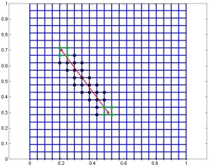
This illustration of the extended finite elements method shows enriched nodes clustered around a crack to capture its movement and characteristics. The two types of marks (circles or squares) indicate which kind of function was used to enrich the nodes.
But “those special functions don’t come for free.” They add degrees

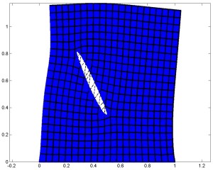
With the extended finite element method, deformed cracks can cut across elements, alleviating the need for special meshing around them.
of freedom – additional properties to calculate at each of the enriched points. “This can result in huge systems of equations that need to be solved repeatedly. It’s very demanding.”
To untangle the equations the researchers plan to apply multigrid methods, techniques that translate the detailed problem to a mesh with fewer data points, making it easier for a computer to solve. Multigrid methods do this by creating a hierarchy of grids, each coarser than the one before it, with each point representing a set of points in the finer grid before it.
Starting with the finest grid, a solver iteratively reduces high-frequency error in the approximate solution. That approximation is projected onto the next, coarser grid. The process repeats through to the coarsest grid, where the equation is solved and the solution is interpolated onto the finest grid. The process repeats until the entire system of equations is solved.
Geometric multigrid methods set up coarse grids based solely on geometry, such as spacing. The ice fracture modelers instead plan to use algebraic multigrid methods, which are based on the matrix of numerical terms that comprise the linear system of equations.
“You can define your set of coarse grids just by extracting that from the linear system,” Waisman says. “Essentially you’re avoiding any geometrical issues that are more difficult to handle.”
But algebraic multigrid methods don’t distinguish between enriched and regular data points. Treating each the same way as the grids are coarsened can destroy many of the technique’s advantages. So the researchers, Waisman says, are developing ways “to tell the multigrid method, ‘Listen, there are special degrees of freedom here. Be careful when you do the coarsening here.’”
The researchers are turning to Scientific Discovery through Advanced Computing (SciDAC), an ASCR-backed program, for tools to develop these techniques. Towards Optimal Petascale Simulations (TOPS), a SciDAC project headed by collaborator David Keyes of Columbia, provides software to solve equations behind the models while focusing on bottlenecks that can bog down computers. To handle multigrid calculations, the ice fracture project will particularly rely on Trilinos, a TOPS-supported software package collaborator Ray Tuminaro of Sandia National Laboratories in California helped develop.
The collaboration includes training Columbia graduate students in computational and earth sciences. Researchers from both institutions will act as co-advisors and students will intern at Sandia.
Going parallel
Another SciDAC project, the Institute for Combinatorial Scientific Computing and Petascale Simulations (CSCAPES, pronounced “seascapes”), will help address one of the last pieces of the ice fracture simulation: parallel processing on high-performance computers.
Parallel processing divvies up a problem among the thousands of processors that comprise today’s supercomputers. Each processor solves its part of the problem and the answers are assembled into the full picture. Parallel computers produce results thousands of times faster than standard, single-processor computers, letting scientists tackle huge problems.
But solving enriched elements can overload some processors while ones calculating conventional elements – those located away from fractures and other unusual features – sit idle. The resulting inefficiencies can slow the calculations.
To balance the computational load, collaborator Erik Boman of Sandia will bring in Zoltan, a CSCAPES tool he helped develop. It will track processor loads and redistribute data on the fly to even out the work.
In the end, Waisman says, “You’re going to have an ice shelf full of networks of cracks, all propagating and interacting. When you model this problem you will have huge systems that need to be solved, so you would need to use algebraic multigrid methods and also solve it on parallel computers. Otherwise it would be almost impossible.”
Eventually, Waisman and his colleagues hope to compare their data with satellite images of ice shelf disintegration to see how accurate their models are. And they’re already meeting with fellow ISICLES researcher Bill Lipscomb of Los Alamos National Laboratory to discuss coupling their code with ice sheet models. Lipscomb is helping develop the Community Ice Sheet Model, which will become part of a global model designed to assess climate change.
Integrating the codes will help eliminate the educated guesses climate researchers now must make about fracturing’s effects, Waisman says. “This is critical to get right, so if we can provide more physics-based fracture calving rates, I think this will be a big improvement.”
